Getting started

This very brief tutorial introduces on how to obtain a likelihood function to fit a bending power-law power spectrum model to some time series data.

As Pioran is written in Julia, you need to install Julia first. Please refer to the official website for the installation.

Installation

Once Julia is installed, you can install Pioran by running the following command in the Julia REPL:

import Pkg; Pkg.add("Pioran")

You may need to install other packages such as Distributions, Plots, DelimitedFiles to run the examples.

Note

Another way to install packages in the Julia REPL is to use the ] key to enter the package manager and then type add MyPackage. See below:

pkg> add Distributions Plots DelimitedFiles

Usage

First, load the package using the following command:

using Pioran

Assuming you have a time series y with measurement error yerr indexed by time t.

using Plots
scatter(t, y,yerr=yerr, label="data",xlabel="Time (days)",ylabel="Value",legend=false,framestyle = :box,ms=3)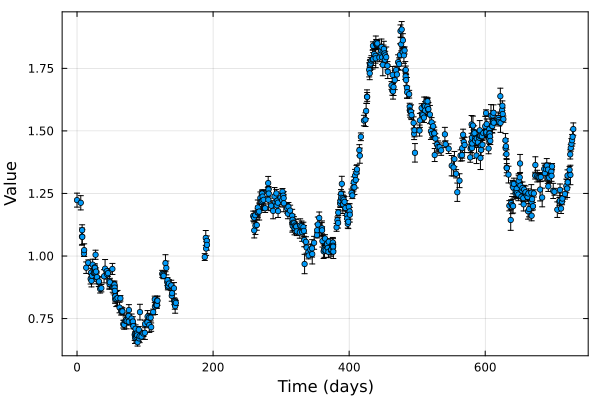

Let's assume we can model the power spectrum with a single-bending power-law model SingleBendingPowerLaw. We can define a power spectral density (PSD) as follows:

α₁, f₁, α₂ = 0.3, 0.03, 3.2
𝓟 = SingleBendingPowerLaw(α₁, f₁, α₂)

SingleBendingPowerLaw{Float64}(1.0, 0.3, 0.03, 3.2)

We can plot the PSD:

f = 10 .^ range(-3, stop=3, length=1000)
plot(f, 𝓟.(f), label="Single Bending Power Law",xlabel="Frequency (day^-1)",ylabel="Power Spectral Density",legend=true,framestyle = :box,xscale=:log10,yscale=:log10)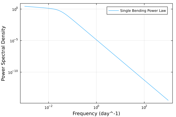

To compute the corresponding covariance function, we need to calculate the inverse Fourier transform of the PSD. However it is very hard, to my knowledge there is no closed form for this integral. We could use the discrete Fourier transform but it would be limiting in terms of performance and one would need to use interpolation to evaluate the function at any given point. Instead, we approximate the PSD model with a sum of basis functions named SHO or DRWCelerite using the approx function.

f_min, f_max = 1/(t[end]-t[1]), 1/2/minimum(diff(t))
norm = 12.3
𝓡 = approx(𝓟, f_min, f_max, 20, norm, basis_function="SHO")

Pioran.SumOfCelerite{StructArrays.StructArray{<:Pioran.SemiSeparable}}(Celerite[Celerite(0.07893716095878586, 0.07893716095878586, 0.0003045156229032465, 0.0003045156229032465), Celerite(0.06483188206344193, 0.06483188206344193, 0.00061247635952396, 0.00061247635952396), Celerite(0.2067393666556462, 0.2067393666556462, 0.001231881922507838, 0.001231881922507838), Celerite(0.137663522918251, 0.137663522918251, 0.002477700644937695, 0.002477700644937695), Celerite(0.625471164721564, 0.625471164721564, 0.004983432562616899, 0.004983432562616899), Celerite(0.21510323198956605, 0.21510323198956605, 0.010023244800331777, 0.010023244800331777), Celerite(1.9875578744664626, 1.9875578744664626, 0.020159886797910555, 0.020159886797910555), Celerite(0.16008466325244336, 0.16008466325244336, 0.040547850900649995, 0.040547850900649995), Celerite(10.066261942432199, 10.066261942432199, 0.08155443674573346, 0.08155443674573346), Celerite(11.934623034122293, 11.934623034122293, 0.16403153324230108, 0.16403153324230108), Celerite(1.5407709359436363, 1.5407709359436363, 0.3299188244253031, 0.3299188244253031), Celerite(0.3048809392182119, 0.3048809392182119, 0.6635701597045385, 0.6635701597045385), Celerite(0.06352139901236725, 0.06352139901236725, 1.334647568586982, 1.334647568586982), Celerite(0.013767817330950088, 0.013767817330950088, 2.684394568207046, 2.684394568207046), Celerite(0.0029416198730311555, 0.0029416198730311555, 5.399158824713996, 5.399158824713996), Celerite(0.0006344173317775932, 0.0006344173317775932, 10.859400611124569, 10.859400611124569), Celerite(0.0001360605960837964, 0.0001360605960837964, 21.84165820295891, 21.84165820295891), Celerite(2.9380708825191376e-5, 2.9380708825191376e-5, 43.93042030019375, 43.93042030019375), Celerite(6.1066621807457676e-6, 6.1066621807457676e-6, 88.35784397954863, 88.35784397954863), Celerite(1.7001080919162074e-6, 1.7001080919162074e-6, 177.71531752633462, 177.71531752633462)], [0.07893716095878586, 0.06483188206344193, 0.2067393666556462, 0.137663522918251, 0.625471164721564, 0.21510323198956605, 1.9875578744664626, 0.16008466325244336, 10.066261942432199, 11.934623034122293, 1.5407709359436363, 0.3048809392182119, 0.06352139901236725, 0.013767817330950088, 0.0029416198730311555, 0.0006344173317775932, 0.0001360605960837964, 2.9380708825191376e-5, 6.1066621807457676e-6, 1.7001080919162074e-6], [0.07893716095878586, 0.06483188206344193, 0.2067393666556462, 0.137663522918251, 0.625471164721564, 0.21510323198956605, 1.9875578744664626, 0.16008466325244336, 10.066261942432199, 11.934623034122293, 1.5407709359436363, 0.3048809392182119, 0.06352139901236725, 0.013767817330950088, 0.0029416198730311555, 0.0006344173317775932, 0.0001360605960837964, 2.9380708825191376e-5, 6.1066621807457676e-6, 1.7001080919162074e-6], [0.0003045156229032465, 0.00061247635952396, 0.001231881922507838, 0.002477700644937695, 0.004983432562616899, 0.010023244800331777, 0.020159886797910555, 0.040547850900649995, 0.08155443674573346, 0.16403153324230108, 0.3299188244253031, 0.6635701597045385, 1.334647568586982, 2.684394568207046, 5.399158824713996, 10.859400611124569, 21.84165820295891, 43.93042030019375, 88.35784397954863, 177.71531752633462], [0.0003045156229032465, 0.00061247635952396, 0.001231881922507838, 0.002477700644937695, 0.004983432562616899, 0.010023244800331777, 0.020159886797910555, 0.040547850900649995, 0.08155443674573346, 0.16403153324230108, 0.3299188244253031, 0.6635701597045385, 1.334647568586982, 2.684394568207046, 5.399158824713996, 10.859400611124569, 21.84165820295891, 43.93042030019375, 88.35784397954863, 177.71531752633462])

The normalisation of the PSD is given using norm which corresponds to the integral of the PSD between f_min and f_max. More details about approximating the power spectral density can be found in the Approximating the power spectral density section of Modelling. We can also plot the autocovariance function:

τ = range(0, stop=300, length=1000)
plot(τ, 𝓡.(τ,0.), label="Covariance function",xlabel="Time lag (days)",ylabel="Autocovariance",legend=true,framestyle = :box)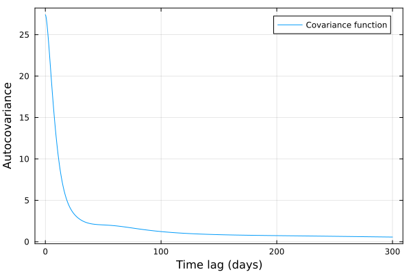

We can now build a Gaussian Process (GP) $f$ which uses the quasi-separable structure of the covariance function to speed up the computations, see Foreman-Mackey et al. (2017). If the mean of the process $\mu$ is known, it can be given as an argument. Otherwise, the mean is assumed to be zero. The GP is constructed as follows:

μ = 1.3
f = ScalableGP(μ, 𝓡)

ScalableGP{AbstractGPs.GP{AbstractGPs.ConstMean{Float64}, Pioran.SumOfCelerite{StructArrays.StructArray{<:Pioran.SemiSeparable}}}, Pioran.SumOfCelerite{StructArrays.StructArray{<:Pioran.SemiSeparable}}, Symbol}(AbstractGPs.GP{AbstractGPs.ConstMean{Float64}, Pioran.SumOfCelerite{StructArrays.StructArray{<:Pioran.SemiSeparable}}}(AbstractGPs.ConstMean{Float64}(1.3), Pioran.SumOfCelerite{StructArrays.StructArray{<:Pioran.SemiSeparable}}(Celerite[Celerite(0.07893716095878586, 0.07893716095878586, 0.0003045156229032465, 0.0003045156229032465), Celerite(0.06483188206344193, 0.06483188206344193, 0.00061247635952396, 0.00061247635952396), Celerite(0.2067393666556462, 0.2067393666556462, 0.001231881922507838, 0.001231881922507838), Celerite(0.137663522918251, 0.137663522918251, 0.002477700644937695, 0.002477700644937695), Celerite(0.625471164721564, 0.625471164721564, 0.004983432562616899, 0.004983432562616899), Celerite(0.21510323198956605, 0.21510323198956605, 0.010023244800331777, 0.010023244800331777), Celerite(1.9875578744664626, 1.9875578744664626, 0.020159886797910555, 0.020159886797910555), Celerite(0.16008466325244336, 0.16008466325244336, 0.040547850900649995, 0.040547850900649995), Celerite(10.066261942432199, 10.066261942432199, 0.08155443674573346, 0.08155443674573346), Celerite(11.934623034122293, 11.934623034122293, 0.16403153324230108, 0.16403153324230108), Celerite(1.5407709359436363, 1.5407709359436363, 0.3299188244253031, 0.3299188244253031), Celerite(0.3048809392182119, 0.3048809392182119, 0.6635701597045385, 0.6635701597045385), Celerite(0.06352139901236725, 0.06352139901236725, 1.334647568586982, 1.334647568586982), Celerite(0.013767817330950088, 0.013767817330950088, 2.684394568207046, 2.684394568207046), Celerite(0.0029416198730311555, 0.0029416198730311555, 5.399158824713996, 5.399158824713996), Celerite(0.0006344173317775932, 0.0006344173317775932, 10.859400611124569, 10.859400611124569), Celerite(0.0001360605960837964, 0.0001360605960837964, 21.84165820295891, 21.84165820295891), Celerite(2.9380708825191376e-5, 2.9380708825191376e-5, 43.93042030019375, 43.93042030019375), Celerite(6.1066621807457676e-6, 6.1066621807457676e-6, 88.35784397954863, 88.35784397954863), Celerite(1.7001080919162074e-6, 1.7001080919162074e-6, 177.71531752633462, 177.71531752633462)], [0.07893716095878586, 0.06483188206344193, 0.2067393666556462, 0.137663522918251, 0.625471164721564, 0.21510323198956605, 1.9875578744664626, 0.16008466325244336, 10.066261942432199, 11.934623034122293, 1.5407709359436363, 0.3048809392182119, 0.06352139901236725, 0.013767817330950088, 0.0029416198730311555, 0.0006344173317775932, 0.0001360605960837964, 2.9380708825191376e-5, 6.1066621807457676e-6, 1.7001080919162074e-6], [0.07893716095878586, 0.06483188206344193, 0.2067393666556462, 0.137663522918251, 0.625471164721564, 0.21510323198956605, 1.9875578744664626, 0.16008466325244336, 10.066261942432199, 11.934623034122293, 1.5407709359436363, 0.3048809392182119, 0.06352139901236725, 0.013767817330950088, 0.0029416198730311555, 0.0006344173317775932, 0.0001360605960837964, 2.9380708825191376e-5, 6.1066621807457676e-6, 1.7001080919162074e-6], [0.0003045156229032465, 0.00061247635952396, 0.001231881922507838, 0.002477700644937695, 0.004983432562616899, 0.010023244800331777, 0.020159886797910555, 0.040547850900649995, 0.08155443674573346, 0.16403153324230108, 0.3299188244253031, 0.6635701597045385, 1.334647568586982, 2.684394568207046, 5.399158824713996, 10.859400611124569, 21.84165820295891, 43.93042030019375, 88.35784397954863, 177.71531752633462], [0.0003045156229032465, 0.00061247635952396, 0.001231881922507838, 0.002477700644937695, 0.004983432562616899, 0.010023244800331777, 0.020159886797910555, 0.040547850900649995, 0.08155443674573346, 0.16403153324230108, 0.3299188244253031, 0.6635701597045385, 1.334647568586982, 2.684394568207046, 5.399158824713996, 10.859400611124569, 21.84165820295891, 43.93042030019375, 88.35784397954863, 177.71531752633462])), Pioran.SumOfCelerite{StructArrays.StructArray{<:Pioran.SemiSeparable}}(Celerite[Celerite(0.07893716095878586, 0.07893716095878586, 0.0003045156229032465, 0.0003045156229032465), Celerite(0.06483188206344193, 0.06483188206344193, 0.00061247635952396, 0.00061247635952396), Celerite(0.2067393666556462, 0.2067393666556462, 0.001231881922507838, 0.001231881922507838), Celerite(0.137663522918251, 0.137663522918251, 0.002477700644937695, 0.002477700644937695), Celerite(0.625471164721564, 0.625471164721564, 0.004983432562616899, 0.004983432562616899), Celerite(0.21510323198956605, 0.21510323198956605, 0.010023244800331777, 0.010023244800331777), Celerite(1.9875578744664626, 1.9875578744664626, 0.020159886797910555, 0.020159886797910555), Celerite(0.16008466325244336, 0.16008466325244336, 0.040547850900649995, 0.040547850900649995), Celerite(10.066261942432199, 10.066261942432199, 0.08155443674573346, 0.08155443674573346), Celerite(11.934623034122293, 11.934623034122293, 0.16403153324230108, 0.16403153324230108), Celerite(1.5407709359436363, 1.5407709359436363, 0.3299188244253031, 0.3299188244253031), Celerite(0.3048809392182119, 0.3048809392182119, 0.6635701597045385, 0.6635701597045385), Celerite(0.06352139901236725, 0.06352139901236725, 1.334647568586982, 1.334647568586982), Celerite(0.013767817330950088, 0.013767817330950088, 2.684394568207046, 2.684394568207046), Celerite(0.0029416198730311555, 0.0029416198730311555, 5.399158824713996, 5.399158824713996), Celerite(0.0006344173317775932, 0.0006344173317775932, 10.859400611124569, 10.859400611124569), Celerite(0.0001360605960837964, 0.0001360605960837964, 21.84165820295891, 21.84165820295891), Celerite(2.9380708825191376e-5, 2.9380708825191376e-5, 43.93042030019375, 43.93042030019375), Celerite(6.1066621807457676e-6, 6.1066621807457676e-6, 88.35784397954863, 88.35784397954863), Celerite(1.7001080919162074e-6, 1.7001080919162074e-6, 177.71531752633462, 177.71531752633462)], [0.07893716095878586, 0.06483188206344193, 0.2067393666556462, 0.137663522918251, 0.625471164721564, 0.21510323198956605, 1.9875578744664626, 0.16008466325244336, 10.066261942432199, 11.934623034122293, 1.5407709359436363, 0.3048809392182119, 0.06352139901236725, 0.013767817330950088, 0.0029416198730311555, 0.0006344173317775932, 0.0001360605960837964, 2.9380708825191376e-5, 6.1066621807457676e-6, 1.7001080919162074e-6], [0.07893716095878586, 0.06483188206344193, 0.2067393666556462, 0.137663522918251, 0.625471164721564, 0.21510323198956605, 1.9875578744664626, 0.16008466325244336, 10.066261942432199, 11.934623034122293, 1.5407709359436363, 0.3048809392182119, 0.06352139901236725, 0.013767817330950088, 0.0029416198730311555, 0.0006344173317775932, 0.0001360605960837964, 2.9380708825191376e-5, 6.1066621807457676e-6, 1.7001080919162074e-6], [0.0003045156229032465, 0.00061247635952396, 0.001231881922507838, 0.002477700644937695, 0.004983432562616899, 0.010023244800331777, 0.020159886797910555, 0.040547850900649995, 0.08155443674573346, 0.16403153324230108, 0.3299188244253031, 0.6635701597045385, 1.334647568586982, 2.684394568207046, 5.399158824713996, 10.859400611124569, 21.84165820295891, 43.93042030019375, 88.35784397954863, 177.71531752633462], [0.0003045156229032465, 0.00061247635952396, 0.001231881922507838, 0.002477700644937695, 0.004983432562616899, 0.010023244800331777, 0.020159886797910555, 0.040547850900649995, 0.08155443674573346, 0.16403153324230108, 0.3299188244253031, 0.6635701597045385, 1.334647568586982, 2.684394568207046, 5.399158824713996, 10.859400611124569, 21.84165820295891, 43.93042030019375, 88.35784397954863, 177.71531752633462]), :celerite)

We can compute the log-likelihood of the Gaussian process given data y, times t and measurement variances σ² using the function logpdf from the Distributions package. f(t, σ²) is the Gaussian process where we incorporate the knowledge of measurement variance σ² and the time values t.

using Distributions
logpdf(f(t, σ²), y)

-340.6597463584629

We can combine all these steps in a function to build the GP and then compute the log-likelihood of the data given the parameters of the power spectral density and the Gaussian process.

function GP_model(t, y, σ, params)

    α₁, f₁, α₂, norm, μ = params

    σ² = σ .^ 2

    # Define power spectral density function
    𝓟 = SingleBendingPowerLaw(α₁, f₁, α₂)

    # Approximation of the PSD to form a covariance function
    𝓡 = approx(𝓟, f_min, f_max, 20, norm, basis_function="SHO")

    # Build the GP
    GP = ScalableGP(μ, 𝓡)

    # sample the conditioned distribution
    return GP(t,σ²)
end

function loglikelihood(t, y, σ, params)
    GP = GP_model(t, y, σ, params)
    return logpdf(GP, y)
end

loglikelihood (generic function with 1 method)