Modelling features in the power spectrum

While this package is designed to model broadband power spectral densities that are power-law-like, we can add narrow features using basis functions.

This feature is currently experimental and may not work properly. Use it at your own risk!

Defining the model and simulating form the model

we defined a power spectral model as sum of two QPOs and a bending power-law.

using Plots
using Pioran
using Random
using Distributions
cont = SingleBendingPowerLaw(0.5,1., 3.6)
q1 =  QPO(7.3,0.1,2)
q2 = QPO(9e-4,2,11)
𝓟 = cont + q1 + q2
f = 10 .^range(-3,1,1000)
p1 = Plots.plot(f,𝓟.(f),xlabel="Frequency (day^-1)",ylabel="Power Spectral Density",legend=true,framestyle = :box,xscale=:log10,yscale=:log10,lw=2,ylim=(1e-5,1e3),label="total")
p1 = Plots.plot!(f,q1.(f),label="QPO1",linestyle=:dash)
Plots.plot!(p1,f,q2.(f),label="QPO2",linestyle=:dot)
Plots.plot!(f,cont.(f),label="cont",linestyle=:dash)
p1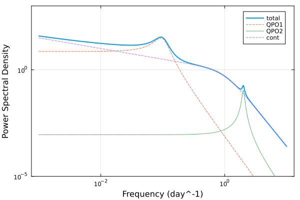

We now simulate time series from this process. To do so we will use the GP method by approximating the bending power-law with basis functions.

t = range(0.,1e3,step=0.1)
yerr = 0.3*ones(length(t));
using QuadGK

In this example power spectrum is normalised by its integral (so its integral is the same as the model after approximation) to make proper comparison with the model.

f_min,f_max = 1/t[end],1/2/diff(t)[1]
norm = quadgk(x->𝓟(x),f_min,f_max,rtol=1e-14)[1]/2

𝓡 = approx(𝓟, f_min, f_max, 35, norm, basis_function="DRWCelerite")
GP = ScalableGP(0.0, 𝓡)
GPc = GP(t,yerr.^2)

AbstractGPs.FiniteGP{ScalableGP{AbstractGPs.GP{AbstractGPs.ConstMean{Float64}, Pioran.SumOfCelerite{StructArrays.StructArray{<:Pioran.SemiSeparable}}}, Pioran.SumOfCelerite{StructArrays.StructArray{<:Pioran.SemiSeparable}}, Symbol}, StepRangeLen{Float64, Base.TwicePrecision{Float64}, Base.TwicePrecision{Float64}, Int64}, LinearAlgebra.Diagonal{Float64, Vector{Float64}}}(
f: ScalableGP{AbstractGPs.GP{AbstractGPs.ConstMean{Float64}, Pioran.SumOfCelerite{StructArrays.StructArray{<:Pioran.SemiSeparable}}}, Pioran.SumOfCelerite{StructArrays.StructArray{<:Pioran.SemiSeparable}}, Symbol}(AbstractGPs.GP{AbstractGPs.ConstMean{Float64}, Pioran.SumOfCelerite{StructArrays.StructArray{<:Pioran.SemiSeparable}}}(AbstractGPs.ConstMean{Float64}(0.0), Pioran.SumOfCelerite{StructArrays.StructArray{<:Pioran.SemiSeparable}}(Celerite[Celerite(0.0009614055938121361, 0.0016652033351635463, 0.00015707963267948965, 0.00027206990463513265), Celerite(0.000943702123654745, 0.0016345400253806655, 0.00024068237516929115, 0.00041687410227956624), Celerite(0.0011991212851879655, 0.0020769389903828456, 0.00036878113813348153, 0.0006387476681202663), Celerite(0.001481605425813006, 0.002566215874277847, 0.0005650581092502792, 0.000978709354450289), Celerite(0.0018327924551438252, 0.0031744896520380073, 0.0008657998845752573, 0.0014996093892716152), Celerite(0.002271144616330877, 0.003933737866821604, 0.0013266059328395682, 0.0022977488773004377), Celerite(0.002807465526403659, 0.00486267293222924, 0.002032667516360898, 0.0035206834132319176), Celerite(0.003481056878954383, 0.006029367378386134, 0.0031145173783633665, 0.005394502340381571), Celerite(0.0042999546321537425, 0.007447739893131424, 0.004772161911404874, 0.008265626892498249), Celerite(0.005336439255850745, 0.009242983922638542, 0.0073120572281508926, 0.0126648546270086)  …  Celerite(0.006048948336661939, 0.0, 31.689033009267337, 0.0), Celerite(0.001991269374271665, 0.0, 48.55493739949656, 0.0), Celerite(0.0006559917555174591, 0.0, 74.39740888210642, 0.0), Celerite(0.00021665253656047155, 0.0, 113.99406002382602, 0.0), Celerite(7.085296004053316e-5, 0.0, 174.66529971907454, 0.0), Celerite(2.42515454439101e-5, 0.0, 267.62768971977687, 0.0), Celerite(6.642219806795628e-6, 0.0, 410.06760026143485, 0.0), Celerite(4.1047060733927795e-6, 0.0, 628.3185307179587, 0.0), Celerite(2.2938494605646897, 0.5922693839649275, 0.15707963267948966, 0.6083668013960418), Celerite(0.031108369396699222, 0.0014154798193870928, 0.5711986642890533, 12.553382114129409)], [0.0009614055938121361, 0.000943702123654745, 0.0011991212851879655, 0.001481605425813006, 0.0018327924551438252, 0.002271144616330877, 0.002807465526403659, 0.003481056878954383, 0.0042999546321537425, 0.005336439255850745  …  0.006048948336661939, 0.001991269374271665, 0.0006559917555174591, 0.00021665253656047155, 7.085296004053316e-5, 2.42515454439101e-5, 6.642219806795628e-6, 4.1047060733927795e-6, 2.2938494605646897, 0.031108369396699222], [0.0016652033351635463, 0.0016345400253806655, 0.0020769389903828456, 0.002566215874277847, 0.0031744896520380073, 0.003933737866821604, 0.00486267293222924, 0.006029367378386134, 0.007447739893131424, 0.009242983922638542  …  0.0, 0.0, 0.0, 0.0, 0.0, 0.0, 0.0, 0.0, 0.5922693839649275, 0.0014154798193870928], [0.00015707963267948965, 0.00024068237516929115, 0.00036878113813348153, 0.0005650581092502792, 0.0008657998845752573, 0.0013266059328395682, 0.002032667516360898, 0.0031145173783633665, 0.004772161911404874, 0.0073120572281508926  …  31.689033009267337, 48.55493739949656, 74.39740888210642, 113.99406002382602, 174.66529971907454, 267.62768971977687, 410.06760026143485, 628.3185307179587, 0.15707963267948966, 0.5711986642890533], [0.00027206990463513265, 0.00041687410227956624, 0.0006387476681202663, 0.000978709354450289, 0.0014996093892716152, 0.0022977488773004377, 0.0035206834132319176, 0.005394502340381571, 0.008265626892498249, 0.0126648546270086  …  0.0, 0.0, 0.0, 0.0, 0.0, 0.0, 0.0, 0.0, 0.6083668013960418, 12.553382114129409])), Pioran.SumOfCelerite{StructArrays.StructArray{<:Pioran.SemiSeparable}}(Celerite[Celerite(0.0009614055938121361, 0.0016652033351635463, 0.00015707963267948965, 0.00027206990463513265), Celerite(0.000943702123654745, 0.0016345400253806655, 0.00024068237516929115, 0.00041687410227956624), Celerite(0.0011991212851879655, 0.0020769389903828456, 0.00036878113813348153, 0.0006387476681202663), Celerite(0.001481605425813006, 0.002566215874277847, 0.0005650581092502792, 0.000978709354450289), Celerite(0.0018327924551438252, 0.0031744896520380073, 0.0008657998845752573, 0.0014996093892716152), Celerite(0.002271144616330877, 0.003933737866821604, 0.0013266059328395682, 0.0022977488773004377), Celerite(0.002807465526403659, 0.00486267293222924, 0.002032667516360898, 0.0035206834132319176), Celerite(0.003481056878954383, 0.006029367378386134, 0.0031145173783633665, 0.005394502340381571), Celerite(0.0042999546321537425, 0.007447739893131424, 0.004772161911404874, 0.008265626892498249), Celerite(0.005336439255850745, 0.009242983922638542, 0.0073120572281508926, 0.0126648546270086)  …  Celerite(0.006048948336661939, 0.0, 31.689033009267337, 0.0), Celerite(0.001991269374271665, 0.0, 48.55493739949656, 0.0), Celerite(0.0006559917555174591, 0.0, 74.39740888210642, 0.0), Celerite(0.00021665253656047155, 0.0, 113.99406002382602, 0.0), Celerite(7.085296004053316e-5, 0.0, 174.66529971907454, 0.0), Celerite(2.42515454439101e-5, 0.0, 267.62768971977687, 0.0), Celerite(6.642219806795628e-6, 0.0, 410.06760026143485, 0.0), Celerite(4.1047060733927795e-6, 0.0, 628.3185307179587, 0.0), Celerite(2.2938494605646897, 0.5922693839649275, 0.15707963267948966, 0.6083668013960418), Celerite(0.031108369396699222, 0.0014154798193870928, 0.5711986642890533, 12.553382114129409)], [0.0009614055938121361, 0.000943702123654745, 0.0011991212851879655, 0.001481605425813006, 0.0018327924551438252, 0.002271144616330877, 0.002807465526403659, 0.003481056878954383, 0.0042999546321537425, 0.005336439255850745  …  0.006048948336661939, 0.001991269374271665, 0.0006559917555174591, 0.00021665253656047155, 7.085296004053316e-5, 2.42515454439101e-5, 6.642219806795628e-6, 4.1047060733927795e-6, 2.2938494605646897, 0.031108369396699222], [0.0016652033351635463, 0.0016345400253806655, 0.0020769389903828456, 0.002566215874277847, 0.0031744896520380073, 0.003933737866821604, 0.00486267293222924, 0.006029367378386134, 0.007447739893131424, 0.009242983922638542  …  0.0, 0.0, 0.0, 0.0, 0.0, 0.0, 0.0, 0.0, 0.5922693839649275, 0.0014154798193870928], [0.00015707963267948965, 0.00024068237516929115, 0.00036878113813348153, 0.0005650581092502792, 0.0008657998845752573, 0.0013266059328395682, 0.002032667516360898, 0.0031145173783633665, 0.004772161911404874, 0.0073120572281508926  …  31.689033009267337, 48.55493739949656, 74.39740888210642, 113.99406002382602, 174.66529971907454, 267.62768971977687, 410.06760026143485, 628.3185307179587, 0.15707963267948966, 0.5711986642890533], [0.00027206990463513265, 0.00041687410227956624, 0.0006387476681202663, 0.000978709354450289, 0.0014996093892716152, 0.0022977488773004377, 0.0035206834132319176, 0.005394502340381571, 0.008265626892498249, 0.0126648546270086  …  0.0, 0.0, 0.0, 0.0, 0.0, 0.0, 0.0, 0.0, 0.6083668013960418, 12.553382114129409]), :celerite)
x: 0.0:0.1:1000.0
Σy: [0.09 0.0 … 0.0 0.0; 0.0 0.09 … 0.0 0.0; … ; 0.0 0.0 … 0.09 0.0; 0.0 0.0 … 0.0 0.09]
)

We can sample realisations from this process:

rng = MersenneTwister(12)
y = [rand(rng,GPc) for i in 1:100]
Plots.plot(t,y[1:3],xlabel="Time",ylabel="Value",legend=false,framestyle = :box,ms=3)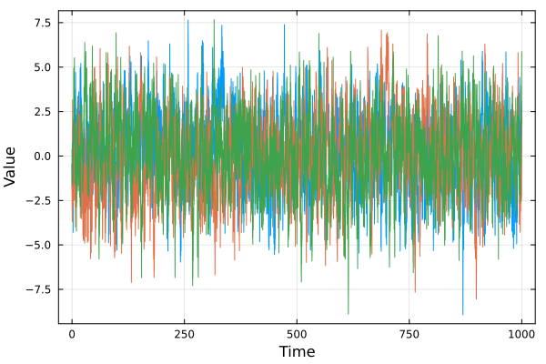

As it is not very informative to look at the time series, let's compute the periodogram using Tonari.jl.

using Tonari
x_GP = mapreduce(permutedims,vcat,y)
fP,I = periodogram(t,x_GP',apply_end_matching=false)

([0.000999900009999, 0.001999800019998, 0.0029997000299970002, 0.003999600039996, 0.004999500049995, 0.0059994000599940004, 0.006999300069993001, 0.007999200079992, 0.008999100089991, 0.00999900009999  …  4.99050094990501, 4.991500849915008, 4.992500749925007, 4.993500649935006, 4.9945005499450055, 4.995500449955005, 4.996500349965004, 4.997500249975002, 4.998500149985001, 4.999500049995], [47.158918780790685, 31.619410701359232, 26.334414392890416, 22.813761933617734, 25.61309815363729, 21.631188458887678, 21.735630877192804, 17.21150334043438, 20.919977005713474, 18.62706226412852  …  0.024250648792226798, 0.022468689479134826, 0.02592744583340088, 0.019456092303547577, 0.025548656336306416, 0.022275069391926184, 0.024284000846524354, 0.022215277775232405, 0.022347186433492126, 0.024696826556816175])

Δt = t[2]-t[1]
noise_level = 2Δt*mean(yerr.^2)

Plots.plot(fP,I,yscale=:log10,xscale=:log10,xlabel="Frequency (Hz)",ylabel="Power",label="Periodogram",framestyle=:box)
Plots.plot!(f,𝓟.(f),label="Model",linewidth=2)
hline!([noise_level],label="Noise level",linewidth=2,linestyle=:dash,ylim=(noise_level/10,1e3),)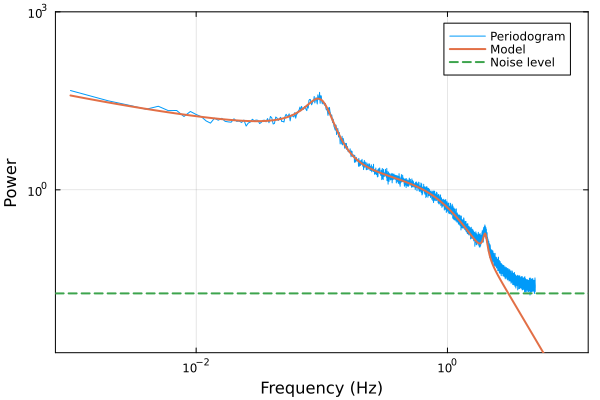

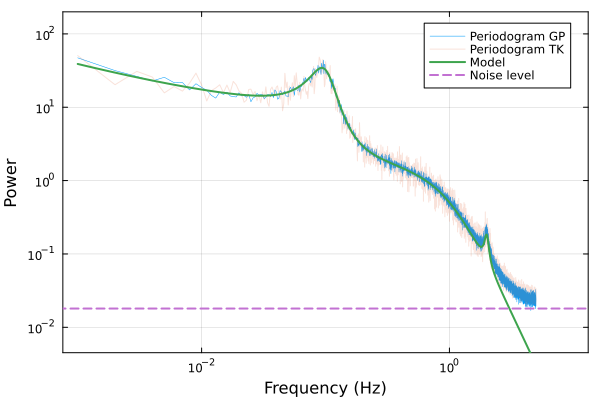
We can even compare the periodogram to the one of simulations using Timmer and König. See the documentation of Tonari.jl for more details:

T, Δt = 504.2, 0.132
simu = Simulation(𝓟, 1e3, 0.1, 20, 20)
rng = MersenneTwister(42)
N = 100
t_TK, x_TK, yerr_TK = sample(rng, simu, N, error_size = 0.25)
fP_TK,I_TK = periodogram(t_TK,x_TK,apply_end_matching=false)

([0.001, 0.002, 0.003, 0.004, 0.005, 0.006, 0.007, 0.008, 0.009000000000000001, 0.01  …  4.9910000000000005, 4.992, 4.993, 4.994, 4.995, 4.996, 4.997, 4.998, 4.999, 5.0], [50.60840630598973, 20.281774070297036, 30.834240939618464, 25.807963999220195, 15.697843014051099, 19.179527178870774, 16.5902728983377, 21.37396707249356, 29.145020347851812, 20.11771612020057  …  0.023900335603256564, 0.022882969906295212, 0.024639147281892895, 0.027820229883572162, 0.02987817536149938, 0.030568122632746844, 0.028762870394919517, 0.02454477593557762, 0.03355210991990242, 0.030121193090363232])

The periodograms agree with the input power spectrum.

Δt = t[2]-t[1]
noise_level = 2Δt*mean(yerr.^2)
noise_level_TK = 2Δt*mean(yerr_TK.^2)

Plots.plot(fP,I,yscale=:log10,xscale=:log10,xlabel="Frequency (Hz)",ylabel="Power",framestyle=:box,label="Periodogram GP",alpha=1,lw=.5)
Plots.plot!(fP_TK,I_TK,label="Periodogram TK",alpha=0.2)
Plots.plot!(f,𝓟.(f),label="Model",linewidth=2)
hline!([noise_level],label="Noise level",linewidth=2,linestyle=:dash,ylim=(noise_level/4,2e2),)